Shares Efficient Frontier
When we invest in a financial instrument (share, index, etc), we usually mostly care about its average annual yield and its variance, which is also called risk or volatility. Naturally, no one can predict the future, so the only thing we can do is to look at the past and assume that the past will reflect the future. So, if we analyze the past history of an instrument, for let’s say 10 or 20 years, we can measure the average annual yield and the variance, or more specifically the standard deviation (which is the square root of the variance, just so it will have the same units as the yield).
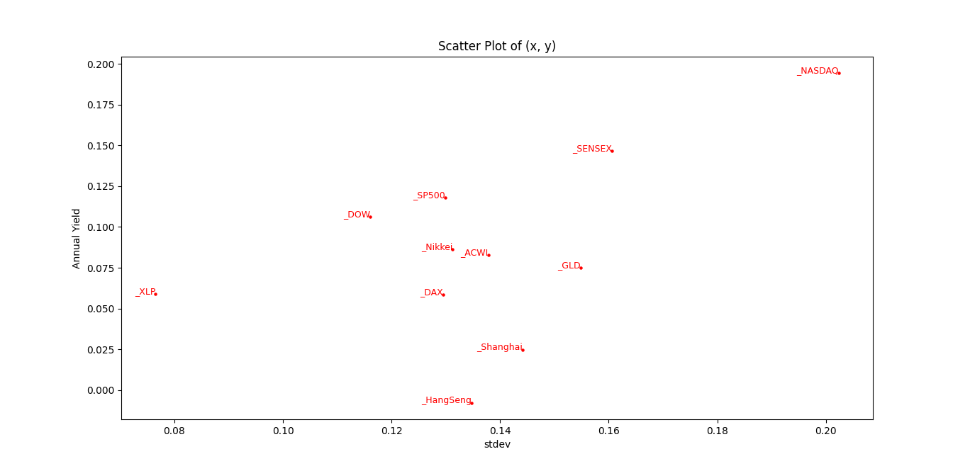
Now, imagine that we plot a map with two axis: the stdev (risk) axis, and the yield, it will look like this:

So we can easily observe, for example, that the NASDAQ has higher yield than the S&P 500, but higher variance. If an instrument has a better yield and lower variance over a second instrument, we would prefer to invest in the first one. This is called a Pareto-better instrument.
Okay. So far, so good. But what happens when we invest in a mixture of instruments? How will the combined coordinate be? So, the combined or weighted average of the yield will simply be the combined weighted average of the individual instruments. But the variance - this is something else. The stdev can sometimes be even lower than each of the instruments. This can happen when the covariance between the instruments is not perfect. In math, when you have two random variables, and you average them together, the resulting stdev is:
\[\frac{1}{2} \sqrt{stdev(X)^2+stdev(Y)^2+2Cov(X,Y)}\]So if $stdev(X)=10=stdev(Y)$ and the variables are independent, meaning their covariance is zero, you get that the combined stdev is 7, which is lower than 10. This is the mathematical grounding for diversifying the risk. You take two risky instruments, invest in both of them, and reduce the risk.
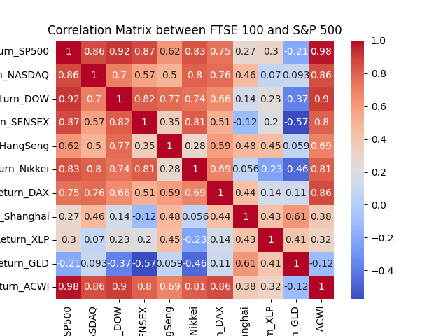
Here you can see the correlation matrix between some instruments:

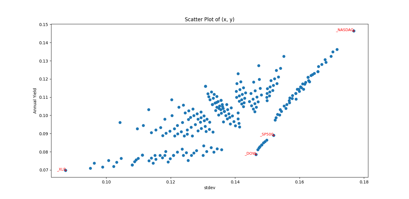
So using this notion, you can invest in a mixture (portfolio) of instruments that will give you pareto-better results, rather than investing in some of the instruments alone, as can be seen here:

So, you can observe many points, that are pareto-better than the Dow Jones or the S&P 500.
\[\square\]Here’s the code:
import pandas as pd
import matplotlib.pyplot as plt
import numpy as np
import seaborn as sns
import mplcursors

val_col_name = 'Close'
base = 4

list_shares = [
				('https://gist.githubusercontent.com/ndvbd/30d8069937f945e492bd440a003296c7/raw/a119c81f4fb3d13d4f5b7b03c6cf0f4d6c778cdf/SP500.csv', 'SP500'),
				('https://gist.githubusercontent.com/ndvbd/2a4516b0f18129287b9de4708f5ce2bf/raw/c69988fc5993699b1bce21c18b4dd1623cb7cb6d/NASDAQ.csv', 'NASDAQ'),
				('https://gist.githubusercontent.com/ndvbd/01cb8aa365e212041037ca44e1068dba/raw/2dc76c20a3a354a641bfa5e0322adc3bc5dfff77/DOW.csv', 'DOW'),
					('https://gist.githubusercontent.com/ndvbd/039f3a31ce29c71cbc8433c9c4d0380e/raw/805b94bde56597caf464c885e681f850d90d6243/XLP.csv', 'XLP'),

]

pandas = []
for i in range(0, len(list_shares)):
	read_df = pd.read_csv(list_shares[i][0], index_col='Date', parse_dates=True)
	first_date = read_df.index[0]
	print(f"first date of {list_shares[i][1]}: {first_date}")
	pandas.append(read_df)

suffixes = [f'_{name[1]}' for name in list_shares]

returns = pandas[0][[val_col_name]].rename(columns={val_col_name: f'{val_col_name}{suffixes[0]}'})
for i in range(1, len(pandas)):
	returns = returns.merge(
		pandas[i][[val_col_name]].rename(columns={val_col_name: f'{val_col_name}{suffixes[i]}'})
		, left_index=True, right_index=True, how='inner')

result = pd.DataFrame()
current_date = returns.index[0]

while current_date <= returns.index[-1]:

	sample = returns.loc[current_date:current_date]

	result = pd.concat([result, sample])

	current_date += pd.DateOffset(years=1)

	if current_date not in returns.index:

		future_dates = returns.index[returns.index >= current_date]
		if len(future_dates) > 0:
			current_date = future_dates[0]
		else:
			break

result = result.reset_index()
returns = result

change_df = returns.copy()

shares_mean_std = []


for i in range(0, len(list_shares)):

	pct_change = change_df[f'Close{suffixes[i]}'].pct_change()
	mean = pct_change[1:].mean()
	stdev = pct_change[1:].std()
	number_years = pct_change.count()
	print(f"For {list_shares[i][1]} we have:  mean: {mean:.3f}, stdev: {stdev:.2f}, number_years: {number_years}")
	shares_mean_std.append((mean, stdev))

	change_df[f'Daily Return{suffixes[i]}'] = pct_change

	change_df.drop(columns=[f'Close{suffixes[i]}'], inplace=True)
change_df.dropna(inplace=True)

to_plot = []

def to_arbitrary_base(number, base, pad_to):
	digits = []
	while number:
		digits.append(int(number % base))
		number //= base

	digits = np.array(digits)
	padded_array = np.pad(digits, (0, pad_to - len(digits)), 'constant')

	return padded_array

def get_composed_earning_for_weight(random_weights):

	list_of_gains = [random_weights]
	current_earning = random_weights.copy()
	for year in range(len(change_df)):
		current_earning = (1 + change_df.iloc[year].values[1:]) * current_earning
		list_of_gains.append(current_earning)

	gain_list = np.array(list_of_gains)
	row_sums = gain_list.sum(axis=1)
	return row_sums

max_base = base ** len(list_shares)
print(f"max_base: {max_base}")
for i in range(max_base):
	if False:
		random_weights = np.random.rand(len(list_shares))
	else:

		random_weights = to_arbitrary_base(i, base=base, pad_to=len(list_shares)) / (base-1.0)
		if random_weights.sum() == 0.0:
			random_weights = np.ones(len(list_shares))

	random_weights = random_weights / random_weights.sum()

	row_sums = get_composed_earning_for_weight(random_weights)

	percent_increase = np.diff(row_sums) / row_sums[:-1]
	mean, std = percent_increase.mean(), percent_increase.std(ddof=1)

	to_plot.append((mean, std, random_weights))

if True:
	y_values, x_values, random_weights = zip(* to_plot)
	plt.scatter(x_values, y_values)

	cursor_hover = mplcursors.cursor(hover=2)
	@cursor_hover.connect("add")
	def on_add(sel):
		index = sel.index
		sel.annotation.set_text(f"[Y{100.0*y_values[index]:.1f}%,{100.0*x_values[index]:.1f}%]=" + str([f"{list_shares[idx][1]}:{val:.2f}" for idx, val in enumerate(random_weights[index]) ]))

	cursor_click = mplcursors.cursor()
	@cursor_click.connect("add")
	def on_click(sel):
		index = sel.index
		weight_vector = [val for idx, val in enumerate(random_weights[index])]
		print(f"plotting mixture: {weight_vector}")
		row_sums = get_composed_earning_for_weight(weight_vector)
		plt.figure()
		plt.plot(row_sums)
		plt.title('Plot of Vector')
		plt.xlabel('year')
		plt.ylabel('value')
		plt.xticks(np.arange(len(row_sums)))
		plt.show()

	additional_y_values, additional_x_values = zip(*shares_mean_std)
	scatter = plt.scatter(additional_x_values, additional_y_values, color='red', label='Additional Points', s=5)

	for (x, y, label) in zip(additional_x_values, additional_y_values, suffixes):
		plt.text(x, y, label, fontsize=9, ha='right', color='red')

	plt.xlabel('stdev')
	plt.ylabel('Annual Yield')
	plt.title('Scatter Plot of (x, y)')
	plt.show()
correlation = change_df.corr()
sns.heatmap(correlation, annot=True, cmap='coolwarm')
plt.title('Correlation Matrix between FTSE 100 and S&P 500')
plt.show()